
Kaggle Housing Prices Competition
Purpose
This notebook was written to document the steps and techniques used to achieve a top 2% ranking on Kaggle’s Housing Prices Competition.
Import Libraries
This notebook uses the following packages. Commented out packages are used later in the notebook but are not explicitly loaded into the namespace.
library(tidyverse)        # used for dataframe manipulation
library(forcats)          # functions for categorical variables
library(simputation)      # for imputing NAs
#library(dlookr)          # for detecting skewness
#library(bestNormalize)   # for normalizing skewed data
#library(h2o)             # for model building
Import Data
I downloaded the training and test sets locally just because, so here I read the files and combine them into one data frame. I didn’t use the test set for anything other than identifying all of the possible factor levels, and combining the data sets made that task easier.
ames_train = read.csv("C:\\Users\\jking\\OneDrive\\Documents\\ML\\data\\ames\\train.csv", stringsAsFactors = F)
ames_test = read.csv("C:\\Users\\jking\\OneDrive\\Documents\\ML\\data\\ames\\test.csv", stringsAsFactors = F)

ames = bind_rows(ames_train %>% mutate(data = 'train'), ames_test %>% mutate(data= 'test'))
Identify and Correct Feature Types
Next, I convert character columns to factors and get a list of the factor names. The MSSubClass feature is numeric, but after reading the data description, it really should be a factor. It also doesn’t make sense to leave MoSold as a number since February isn’t two times greater then January. I also will convert YrSold to a factor, but not yet since I’ll do some math with it first.
ames = ames %>% mutate_if(is_character, as_factor)

# convert from number to factor
ames$MSSubClass = as.factor(ames$MSSubClass)
ames$MoSold = as.factor(ames$MoSold)
Numeric Features
I’ll start with the numeric features, which have quite a few missing values. My strategy for replacing the NAs is in the code comments.
# impute NAs as a function of LotArea grouped by Neighborhood
ames = impute_median(ames, LotFrontage ~ Neighborhood)

# replace NAs with 0
ames[is.na(ames$MasVnrArea), 'MasVnrArea'] = 0
ames[is.na(ames$BsmtFinSF1), 'BsmtFinSF1'] = 0
ames[is.na(ames$BsmtFinSF2), 'BsmtFinSF2'] = 0
ames[is.na(ames$BsmtUnfSF), 'BsmtUnfSF'] = 0
ames[is.na(ames$TotalBsmtSF), 'TotalBsmtSF'] = 0
ames[is.na(ames$BsmtFullBath), 'BsmtFullBath'] = 0
ames[is.na(ames$BsmtHalfBath), 'BsmtHalfBath'] = 0
ames[is.na(ames$GarageCars), 'GarageCars'] = 0
ames[is.na(ames$GarageArea), 'GarageArea'] = 0
ames[is.na(ames$GarageYrBlt), 'GarageYrBlt'] = 0
With the NAs taken care of, I created new features that I thought might improve the model performance.
ames = ames %>% mutate(
  TotalPorchSF = OpenPorchSF + EnclosedPorch + X3SsnPorch + ScreenPorch + WoodDeckSF,
  Baths = FullBath + 0.5*HalfBath + BsmtFullBath + 0.5*BsmtHalfBath,
  AgeWhenSold = YrSold - YearBuilt,
  AgeOfRemodel = YrSold - YearRemodAdd,
  TotalWalledArea = TotalBsmtSF + GrLivArea,
  TotalOccupiedArea = TotalPorchSF + TotalWalledArea,
  OtherRooms = TotRmsAbvGrd - BedroomAbvGr - KitchenAbvGr,
  LotDepth = LotArea / LotFrontage,
  TotalSF = TotalBsmtSF + X1stFlrSF + X2ndFlrSF,
)
Now that I’m done with mathematical operations using YrSold , I convert it to a factor.
ames$YrSold = as.factor(ames$YrSold)
Next, I find the features that contain the same value in more than 99.5% of the observations. These will provide virtually no information to help explain why SalesPrice varies, so I drop the features. Turns out there’s just one: PoolArea.
(to_drop = colnames(ames)[which(ames %>% summarise_all(funs(sum(.==0))) / nrow(ames) >0.995)])
## [1] "PoolArea"
ames = ames %>% select(-all_of(to_drop))
The last step is to normalize the numeric features that have a skewed distribution.
sk = dlookr::find_skewness(ames, thres = 0.5)

for (i in sk){ames[, i] = bestNormalize::bestNormalize(ames[, i])$x.t}
Categorical Features
The first step for the categorical features is to replace the NAs using the following strategy:
-
MSZoning: impute missing values using k-nearest neighbors grouped byMSSubClass. -
Exterior1stthroughSaleType: these each have only one missing value, so I impute missing values using the mode. Oddly, R doesn’t have a built-in mode function, so I wrote my own. -
All others: replace missing values with a new level.
# impute missing MSZoning values using KNN grouped by MSSubclass
ames = impute_knn(ames, MSZoning~. -SalePrice | MSSubClass)

# replace with mode of feature
Mode <- function(x) {
    ux <- unique(x)
    return(as.character(ux[which.max(tabulate(match(x, ux)))]))}

ames$Exterior1st = forcats::fct_explicit_na(ames$Exterior1st, Mode(ames$Exterior1st))
ames$Exterior2nd = forcats::fct_explicit_na(ames$Exterior2nd, Mode(ames$Exterior2nd))
ames$Electrical = forcats::fct_explicit_na(ames$Electrical, Mode(ames$Electrical))
ames$KitchenQual = forcats::fct_explicit_na(ames$KitchenQual, Mode(ames$KitchenQual))
ames$Functional = forcats::fct_explicit_na(ames$Functional, Mode(ames$Functional))
ames$SaleType = forcats::fct_explicit_na(ames$SaleType, Mode(ames$SaleType))

# replace other missing NAs
ames$Alley = forcats::fct_explicit_na(ames$Alley, 'Missing')
ames$MasVnrType = forcats::fct_explicit_na(ames$MasVnrType, 'None')
ames$GarageType = forcats::fct_explicit_na(ames$GarageType, "None")
ames$MiscFeature = forcats::fct_explicit_na(ames$MiscFeature, na_level="Missing")
ames$Fence = forcats::fct_explicit_na(ames$Fence, 'None')
Quite a few of the categorical features are Likert-scale responses, so I convert them to integers and group levels when there are less than five. Also, h2o, which I later use for model building, doesn’t recognize R’s ordered factor data type, so integers it is.
ames = ames %>% mutate(ExterQual = case_when(ExterQual == 'Fa' ~ 1,
                                             ExterQual == 'Po' ~ 1,
                                             ExterQual == 'TA' ~ 2,
                                             ExterQual == 'Gd' ~ 3,
                                             ExterQual == 'Ex' ~ 4))

ames = ames %>% mutate(ExterCond = case_when(ExterCond == 'Po' ~ 1,
                                             ExterCond == 'Fa' ~ 1,
                                             ExterCond == 'TA' ~ 2,
                                             ExterCond == 'Gd' ~ 3,
                                             ExterCond == 'Ex' ~ 3))

ames = ames %>% mutate(BsmtQual = case_when(is.na(BsmtQual) ~ 0,
                                            BsmtQual == 'Fa' ~ 1,
                                            BsmtQual == 'TA' ~ 2,
                                            BsmtQual == 'Gd' ~ 3,
                                            BsmtQual == 'Ex' ~ 4),
                       BsmtCond = case_when(is.na(BsmtCond) ~ 0,
                                            BsmtCond == 'Po' ~ 1,
                                            BsmtCond == 'Fa' ~ 1,
                                            BsmtCond == 'TA' ~ 2,
                                            BsmtCond == 'Gd' ~ 3,
                                            BsmtCond == 'Ex' ~ 4),
                       BsmtExposure = case_when(is.na(BsmtExposure) ~ 0,
                                                BsmtExposure == 'No' ~ 1,
                                                BsmtExposure == 'Mn' ~ 2,
                                                BsmtExposure == 'Av' ~ 3,
                                                BsmtExposure == 'Gd' ~ 4),
                       BsmtFinType1 = case_when(is.na(BsmtFinType1) ~ 0,
                                                BsmtFinType1 == 'Unf' ~ 1,
                                                BsmtFinType1 == 'LwQ' ~ 2,
                                                BsmtFinType1 == 'Rec' ~ 3,
                                                BsmtFinType1 == 'BLQ' ~ 4,
                                                BsmtFinType1 == 'ALQ' ~ 5,
                                                BsmtFinType1 == 'GLQ' ~ 6),
                       BsmtFinType2 = case_when(is.na(BsmtFinType2) ~ 0,
                                                BsmtFinType2 == 'Unf' ~ 1,
                                                BsmtFinType2 == 'LwQ' ~ 2,
                                                BsmtFinType2 == 'Rec' ~ 3,
                                                BsmtFinType2 == 'BLQ' ~ 4,
                                                BsmtFinType2 == 'ALQ' ~ 5,
                                                BsmtFinType2 == 'GLQ' ~ 6))

ames = ames %>% mutate(HeatingQC = case_when(HeatingQC == 'Po' ~ 1,
                                             HeatingQC == 'Fa' ~ 1,
                                             HeatingQC == 'TA' ~ 2,
                                             HeatingQC == 'Gd' ~ 3,
                                             HeatingQC == 'Ex' ~ 4))

ames = ames %>% mutate(KitchenQual = case_when(is.na(KitchenQual) ~ 0,
                                               KitchenQual == 'Fa' ~ 1,
                                               KitchenQual == 'TA' ~ 2,
                                               KitchenQual == 'Gd' ~ 3,
                                               KitchenQual == 'Ex' ~ 4))

ames = ames %>% mutate(Functional = case_when(is.na(Functional) ~ 0,
                                              Functional == 'Sev' ~ 1,
                                              Functional == 'Maj2' ~ 1,
                                              Functional == 'Maj1' ~ 2,
                                              Functional == 'Mod' ~ 3,
                                              Functional == 'Min2' ~ 4,
                                              Functional == 'Min1' ~ 5,
                                              Functional == 'Typ' ~ 6))

ames = ames %>% mutate(FireplaceQu = case_when(is.na(FireplaceQu) ~ 0,
                                               FireplaceQu == 'Po' ~ 1,
                                               FireplaceQu == 'Fa' ~ 2,
                                               FireplaceQu == 'TA' ~ 3,
                                               FireplaceQu == 'Gd' ~ 4,
                                               FireplaceQu == 'Ex' ~ 5))

ames = ames %>% mutate(GarageFinish = case_when(is.na(GarageFinish) ~ 0,
                                                GarageFinish == 'Unf' ~ 1,
                                                GarageFinish == 'RFn' ~ 2,
                                                GarageFinish == 'Fin' ~ 3))

ames = ames %>% mutate(GarageQual = case_when(is.na(GarageQual) ~ 0,
                                              GarageQual == 'Po' ~ 1,
                                              GarageQual == 'Fa' ~ 1,
                                              GarageQual == 'TA' ~ 2,
                                              GarageQual == 'Gd' ~ 3,
                                              GarageQual == 'Ex' ~ 3))

ames = ames %>% mutate(GarageCond = case_when(is.na(GarageCond) ~ 0,
                                              GarageCond == 'Po' ~ 1,
                                              GarageCond == 'Fa' ~ 2,
                                              GarageCond == 'TA' ~ 3,
                                              GarageCond == 'Gd' ~ 4,
                                              GarageCond == 'Ex' ~ 4))
As with the numeric features, I don’t want to have a factor level that appears in less than 0.5% of the data, so for each feature, I lumped them into a single level.
factor_cols = colnames(ames %>% select_if(is.factor))

for (fac in factor_cols){
  ames[ , fac] = fct_lump_prop(ames[, fac], prop=0.005)
}
Then I created a couple of new categorical features to describe total garage and exterior quality. I tried several other new categorical features but they turned out to not be useful.
ames$TotalGarageQual = ames$GarageQual * ames$GarageCond
ames$TotalExteriorQual = ames$ExterQual * ames$ExterCond
Unusual Observations
The final step was to identify and drop unusual observations from the training data set. I took a simple approach of fitting a linear model to the numeric features and dropping the observations with a Cook’s distance > 0.5.
df = ames %>% filter(data=='train') %>% select(-all_of(factor_cols))

df.lm = lm(SalePrice ~ ., data=df)
plot(df.lm, which =4)
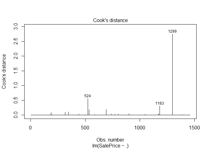
ames = ames %>% filter(!Id %in% c(524, 1299))
A final scrub of the features revealed that four more features would be dropped. Id is just the row number, so of no use. The other three contained a single level that dominated the feature, just not at the 99.5% threshold I used earlier. I then split the data back into separate training and test sets. I also noticed that the response variable distribution was a little skewed, so transformed it using the log of the response.
# drop factors
train_test = ames %>% select(-Id, -Street, -Utilities, -PoolQC)

# split back into train and test sets
train_df = train_test %>% filter(data=='train') %>% select(-SalePrice, everything()) %>% select(-data)
test_df = train_test %>% filter(data=='test') %>% select(-data, -SalePrice)

# transform the response to correct skewness
train_df$SalePrice = log(train_df$SalePrice)

#
# Model
#
library(h2o)
h2o.init()
##  Connection successful!
##
## R is connected to the H2O cluster:
##     H2O cluster uptime:         2 hours 50 minutes
##     H2O cluster timezone:       America/Chicago
##     H2O data parsing timezone:  UTC
##     H2O cluster version:        3.30.0.1
##     H2O cluster version age:    3 months and 25 days !!!
##     H2O cluster name:           H2O_started_from_R_jking_czc335
##     H2O cluster total nodes:    1
##     H2O cluster total memory:   3.11 GB
##     H2O cluster total cores:    8
##     H2O cluster allowed cores:  8
##     H2O cluster healthy:        TRUE
##     H2O Connection ip:          localhost
##     H2O Connection port:        54321
##     H2O Connection proxy:       NA
##     H2O Internal Security:      FALSE
##     H2O API Extensions:         Amazon S3, Algos, AutoML, Core V3, TargetEncoder, Core V4
##     R Version:                  R version 4.0.0 (2020-04-24)
# convert data to h2o frames
train_full = as.h2o(train_df)
##
  |
  |                                                                      |   0%
  |
  |======================================================================| 100%
test_set = as.h2o(test_df)
##
  |
  |                                                                      |   0%
  |
  |======================================================================| 100%
I used h2o’s automl() function to fit an array of distributed random forests, gradient boosted machines, and generalized linear models and also fit some ensembles models. The best performing model turned out to be a generalized linear model, which I didn’t expect.
aml = h2o.automl(x = 1:86, y = 87,
                 training_frame = train_full,
                 exclude_algos = "DeepLearning",
                 nfolds = 10,
                 seed=1)
##
  |
  |                                                                      |   0%
## 13:47:22.23: AutoML: XGBoost is not available; skipping it.
  |
  |=======                                                               |  11%
  |
  |========                                                              |  11%
  |
  |========                                                              |  12%
  |
  |=========                                                             |  12%
  |
  |============                                                          |  17%
  |
  |================                                                      |  22%
  |
  |=================                                                     |  24%
  |
  |=====================                                                 |  29%
  |
  |=========================                                             |  36%
  |
  |==========================                                            |  37%
  |
  |=============================                                         |  42%
  |
  |==============================                                        |  43%
  |
  |==================================                                    |  48%
  |
  |==================================                                    |  49%
  |
  |===================================                                   |  49%
  |
  |===================================                                   |  50%
  |
  |===================================                                   |  51%
  |
  |====================================                                  |  51%
  |
  |=============================================================         |  88%
  |
  |======================================================================| 100%
# aml@leader
# best yet!
# Mean Residual Deviance :  0.009144619

# View the AutoML Leaderboard
lb <- aml@leaderboard
print(lb, n = nrow(lb))
##                                               model_id mean_residual_deviance
## 1                         GLM_1_AutoML_20200729_134722             0.01234028
## 2           GBM_grid__1_AutoML_20200729_134722_model_1             0.01421023
## 3           GBM_grid__1_AutoML_20200729_134722_model_8             0.01424621
## 4          GBM_grid__1_AutoML_20200729_134722_model_17             0.01429914
## 5           GBM_grid__1_AutoML_20200729_134722_model_9             0.01433740
## 6          GBM_grid__1_AutoML_20200729_134722_model_16             0.01450047
## 7          GBM_grid__1_AutoML_20200729_134722_model_14             0.01464563
## 8                         GBM_2_AutoML_20200729_134722             0.01466961
## 9                         GBM_1_AutoML_20200729_134722             0.01472922
## 10          GBM_grid__1_AutoML_20200729_134722_model_6             0.01481323
## 11         GBM_grid__1_AutoML_20200729_134722_model_10             0.01487122
## 12         GBM_grid__1_AutoML_20200729_134722_model_12             0.01492296
## 13          GBM_grid__1_AutoML_20200729_134722_model_7             0.01496287
## 14          GBM_grid__1_AutoML_20200729_134722_model_5             0.01499472
## 15                        GBM_3_AutoML_20200729_134722             0.01503074
## 16         GBM_grid__1_AutoML_20200729_134722_model_11             0.01504675
## 17                        GBM_4_AutoML_20200729_134722             0.01523721
## 18          GBM_grid__1_AutoML_20200729_134722_model_2             0.01557706
## 19          GBM_grid__1_AutoML_20200729_134722_model_4             0.01584540
## 20         GBM_grid__1_AutoML_20200729_134722_model_13             0.01591883
## 21                        GBM_5_AutoML_20200729_134722             0.01709624
## 22                        DRF_1_AutoML_20200729_134722             0.01713740
## 23          GBM_grid__1_AutoML_20200729_134722_model_3             0.01757300
## 24                        XRT_1_AutoML_20200729_134722             0.01759224
## 25         GBM_grid__1_AutoML_20200729_134722_model_15             0.01794169
## 26    StackedEnsemble_AllModels_AutoML_20200729_134722             0.06526690
## 27 StackedEnsemble_BestOfFamily_AutoML_20200729_134722             0.06526690
##         rmse        mse        mae       rmsle
## 1  0.1110868 0.01234028 0.07731224 0.008684675
## 2  0.1192067 0.01421023 0.08140197 0.009299560
## 3  0.1193575 0.01424621 0.08090909 0.009337949
## 4  0.1195790 0.01429914 0.08105349 0.009339289
## 5  0.1197389 0.01433740 0.08346038 0.009342298
## 6  0.1204179 0.01450047 0.08031451 0.009420327
## 7  0.1210191 0.01464563 0.08242345 0.009463250
## 8  0.1211182 0.01466961 0.08272041 0.009469219
## 9  0.1213640 0.01472922 0.08298042 0.009464897
## 10 0.1217096 0.01481323 0.08331827 0.009522902
## 11 0.1219476 0.01487122 0.08270787 0.009524518
## 12 0.1221596 0.01492296 0.08224788 0.009547986
## 13 0.1223228 0.01496287 0.08283091 0.009553652
## 14 0.1224529 0.01499472 0.08148624 0.009573547
## 15 0.1225999 0.01503074 0.08419082 0.009582162
## 16 0.1226652 0.01504675 0.08355947 0.009582873
## 17 0.1234391 0.01523721 0.08536511 0.009644123
## 18 0.1248081 0.01557706 0.08548639 0.009758218
## 19 0.1258785 0.01584540 0.08589779 0.009812402
## 20 0.1261698 0.01591883 0.08537606 0.009873776
## 21 0.1307526 0.01709624 0.08863226 0.010194963
## 22 0.1309099 0.01713740 0.08975185 0.010222975
## 23 0.1325632 0.01757300 0.09070271 0.010321361
## 24 0.1326357 0.01759224 0.09152691 0.010349223
## 25 0.1339466 0.01794169 0.09101699 0.010456578
## 26 0.2554739 0.06526690 0.19248233 0.019648052
## 27 0.2554739 0.06526690 0.19248233 0.019648052
##
## [27 rows x 6 columns]
Lastly, I used the best performing model to make predictions on the test set (after un-doing the log transformation), and submitted those predictions to the Kaggle competition.
aml_preds = exp(h2o.predict(aml@leader, newdata = test_set))
##
  |
  |                                                                      |   0%
  |
  |======================================================================| 100%
submisn = tibble(
  Id = 1461:2919,
  SalePrice = as.vector(aml_preds)
)

head(submisn)
## # A tibble: 6 x 2
##      Id SalePrice
##   <int>     <dbl>
## 1  1461   119968.
## 2  1462   158017.
## 3  1463   183189.
## 4  1464   198801.
## 5  1465   194161.
## 6  1466   168961.
h2o.shutdown(prompt=FALSE)


Comments