
Simple Rating System
Motivation
In my last post, I was playing around with data from an API offered by http://collegefootballdata.com.
Then I found some blog posts on the site, and I thought a couple of them on how Simple Rating Systems work were interesting.
In particular, this one.
They did all their coding in Python, but I’m becoming more and more of an R fan, so I thought I’d re-code the wheel, so to speak.
In their post, they used data from the 2019 season, so for consistency, I’ll do the same.
Also, in the last post, I was using tidyr to un-nest JSON data.
It seemed add to me that you have to do these repeated unnest_auto() steps to get things parsed out.
If it’s automatic, why do I have to keep doing it manually?
After some more Googling, I found the tidyjson package, which has a nice spread_all function that I’ll use instead.
Simple Rating System: The Math
This, to me, is the coolest part.
I had no idea this is how some rating systems work, and it’s pretty slick.
It’s just one big system of equations that you solve with regular ‘ol linear algebra.
In other words, solve .
That’s it.
I’ll start with the b vector - that’s easiest to explain.
The b Vector
The b vector is each team’s average margin of victory for the season.
Couldn’t be any simpler.
The A Matrix
This is a little more complicated.
The A matrix will have dimensions of 130x130 - one row and column for each FBS team.
The diagonal will be 1’s (i.e., the identity matrix).
Think of the rest of the matrix in terms of rows.
We’ll set it up alphabetically, so the first row will be for Air Force.
First, we’ll count how many games Air Force played that season.
Then we’ll identify all of Air Force’s opponents - those are the columns.
As I said, the Air Force-Air Force entry will have a 1.
Moving across the columns, if Air Force didn’t play that team, put a 0 there.
If they did, divide the number of times Air Force played that team by the total number of games played and put that value in the column.
Keep doing that until you get to the last column (i.e., that last potential match-up).
Then repeat that process for the next team, Akron, and then the next, etc.
That’s it.
This matrix represents each team’s strength of schedule.
Pretty clever, right?
A teams rating is it’s mean margin of victory adjusted by it’s strength of schedule.
The Code
First we need to get all the FBS team names so we can exclude non-FBS games.
library(tidyjson)
library(dplyr)
library(httr)

fbs <-
  httr::GET(
    url = "https://api.collegefootballdata.com/teams/fbs?year=2019",
    httr::add_headers(
      Authorization = paste("Bearer", Sys.getenv("YOUR_API_TOKEN"))
    )
  )

fbs_teams <-
  httr::content(fbs, "parsed") %>% # convert response to a nested list
  spread_all %>% # rectangularize nested list into a dataframe
  arrange(school) # make sure teams are in alphabetical order
Now we’ll get team win-loss records.
records <-
  httr::GET(
  url = "https://api.collegefootballdata.com/games?year=2019",
  httr::add_headers(
    accept = "application/json",
    Authorization = paste("Bearer", Sys.getenv("YOUR_API_TOKEN"))
  )
)

team_records <-
  httr::content(records, "parsed") %>%
  spread_all
Now get scores and margin of victory for each game and eliminate non-FBS games.
Eventually we’ll use this for the $b$ vector, but first we’ll need it in this format for the A matrix.
scores <- team_records %>%
  filter(home_team %in% (fbs_teams %>% .$school) & away_team %in% (fbs_teams %>% .$school)) %>%
  select(home_team, away_team, home_points, away_points) %>%
  mutate(home_mov = home_points - away_points)
head(scores)
## # A tbl_json: 6 x 6 tibble with a "JSON" attribute
##   ..JSON                 home_team  away_team   home_points away_points home_mov
##   <chr>                  <chr>      <chr>             <dbl>       <dbl>    <dbl>
## 1 "{\"id\":401110723..." Florida    Miami                24          20        4
## 2 "{\"id\":401114164..." Hawai'i    Arizona              45          38        7
## 3 "{\"id\":401117854..." Cincinnati UCLA                 24          14       10
## 4 "{\"id\":401111653..." Clemson    Georgia Te~          52          14       38
## 5 "{\"id\":401114236..." Tulane     Florida In~          42          14       28
## 6 "{\"id\":401110731..." Texas A&M  Texas State          41           7       34
Ok, now we can start to generate the A matrix.
First, I’ll populate it with the number of times each team faced each other.
There’s probably a more elegant way, but this is what came to me first.
A <- data.frame(diag(0, nrow=130, ncol=130), row.names = fbs_teams %>% .$school)
colnames(A) <- fbs_teams %>% .$school

# populate dataframe with
for (r in 1:nrow(scores)){
  home <- scores[r, 1] %>% .$home_team
  away <- scores[r, 2] %>% .$away_team
  A[home, away] <- A[home, away] + 1
  A[away, home] <- A[away, home] + 1
}

# clean up
rm(away, home, r)

A[1:6, 1:6]
##                   Air Force Akron Alabama Appalachian State Arizona
## Air Force                 0     0       0                 0       0
## Akron                     0     0       0                 0       0
## Alabama                   0     0       0                 0       0
## Appalachian State         0     0       0                 0       0
## Arizona                   0     0       0                 0       0
## Arizona State             0     0       0                 0       1
##                   Arizona State
## Air Force                     0
## Akron                         0
## Alabama                       0
## Appalachian State             0
## Arizona                       1
## Arizona State                 0
Hold that thought on the A matrix - we need a little more work to proceed.
Next, rearrange the scores data to get one margin of victory score for each team and each game.
mov <- scores %>%
  select(home_team, home_mov) %>%
  rename(team = home_team, mov = home_mov) %>%
  bind_rows(scores %>%
              select(away_team, home_mov) %>%
              rename(team = away_team, mov = home_mov) %>%
              mutate(mov = -mov))
Now count the total number of games each team played.
n_games <- mov %>% count(team) %>% .$n
Multiply A’s columns by 1 / n_games.
MARGIN=1 specifies to sweep across columns.
A <- sweep(A, 1/n_games, MARGIN=1, FUN =`*`)
Finally, add the identity matrix and A is built.
A <- A + diag(1, nrow=130, ncol=130)
A[1:6, 1:6]
##                   Air Force Akron Alabama Appalachian State    Arizona
## Air Force                 1     0       0                 0 0.00000000
## Akron                     0     1       0                 0 0.00000000
## Alabama                   0     0       1                 0 0.00000000
## Appalachian State         0     0       0                 1 0.00000000
## Arizona                   0     0       0                 0 1.00000000
## Arizona State             0     0       0                 0 0.09090909
##                   Arizona State
## Air Force            0.00000000
## Akron                0.00000000
## Alabama              0.00000000
## Appalachian State    0.00000000
## Arizona              0.09090909
## Arizona State        1.00000000
Now calculate the mean margin of victory for each team.
This is the $b$ vector for the system of equations.
b <-
  mov %>%
  group_by(team) %>%
  summarize(mean_mov = mean(mov)) %>%
  .$mean_mov
It took a while to build the system of equations, but solving it is a one-liner.
solve(A, b)
##             Air Force                 Akron               Alabama
##           12.17488262          -22.66408637           32.60720600
##     Appalachian State               Arizona         Arizona State
##           21.80515687          -13.03736947            1.10205537
##              Arkansas        Arkansas State                  Army
##          -24.46835876           -0.52637216            1.05006201
##                Auburn            Ball State                Baylor
##            5.88613703            0.40799928           14.36295601
##           Boise State        Boston College         Bowling Green
##           17.32564683           -2.78480549          -33.10414546
##               Buffalo                   BYU            California
##           10.20151104            0.46092289           -6.46928285
##      Central Michigan             Charlotte            Cincinnati
##           10.31277888           -4.34284716            7.36008829
##               Clemson      Coastal Carolina              Colorado
##           41.48627376            0.83014089          -11.45324149
##        Colorado State           Connecticut                  Duke
##           -2.51297888          -22.92597291          -10.33694277
##         East Carolina      Eastern Michigan               Florida
##          -12.21872118           -2.75282448           12.69160016
##      Florida Atlantic Florida International         Florida State
##            8.62463543            1.37276246           -6.07744689
##          Fresno State               Georgia      Georgia Southern
##            0.50823966           15.23789346           -1.56619791
##         Georgia State          Georgia Tech               Hawai'i
##           -2.53872623          -20.00376049            0.03002992
##               Houston              Illinois               Indiana
##          -11.22633847            5.83248366            6.84673009
##                  Iowa            Iowa State                Kansas
##           10.19598383            8.32429892          -17.55664637
##          Kansas State            Kent State              Kentucky
##            9.86298135           -0.90629641           11.16790944
##               Liberty             Louisiana      Louisiana Monroe
##           11.38026279           14.12089636          -10.96010135
##        Louisiana Tech            Louisville                   LSU
##           19.83837303          -11.11555104           24.61782878
##              Marshall              Maryland               Memphis
##           -4.53506310          -21.13126417           16.67762020
##                 Miami            Miami (OH)              Michigan
##            3.40729287           -9.17435086            9.40439559
##        Michigan State      Middle Tennessee             Minnesota
##           -2.84667123           -5.41633827           14.54830499
##     Mississippi State              Missouri                  Navy
##          -10.04679640            5.12551526           14.51847575
##              NC State              Nebraska                Nevada
##          -10.13346295           -1.06634224          -10.70442169
##            New Mexico      New Mexico State        North Carolina
##          -18.96441796          -26.88151749            1.61200847
##           North Texas     Northern Illinois          Northwestern
##           -1.33040741           -5.75767308           -9.39415805
##            Notre Dame                  Ohio            Ohio State
##           21.22221810           10.59616933           36.35622851
##              Oklahoma        Oklahoma State          Old Dominion
##           15.82512098            3.23809017          -14.57638255
##              Ole Miss                Oregon          Oregon State
##           -0.47404615           20.18886699           -6.91414098
##            Penn State            Pittsburgh                Purdue
##           13.07833337           -4.24030653           -4.44792009
##                  Rice               Rutgers       San Diego State
##           -7.94447288          -27.74865910           11.75886571
##        San José State                   SMU         South Alabama
##           -0.51222213           14.52255973          -17.50751350
##        South Carolina         South Florida  Southern Mississippi
##          -20.16977658          -15.55091539           -3.01895055
##              Stanford              Syracuse                   TCU
##          -10.41277836           -5.93538233           -1.45957680
##                Temple             Tennessee                 Texas
##            2.25488829           -4.03217697            1.54246752
##             Texas A&M           Texas State            Texas Tech
##            0.24533392          -19.98074165           -2.56724537
##                Toledo                  Troy                Tulane
##           -9.23735051           -1.27992009           -1.44073888
##                 Tulsa                   UAB                   UCF
##           -9.98788905            7.89737667           22.70582261
##                  UCLA                 UMass                  UNLV
##           -9.73407669          -28.89607277          -12.08819590
##                   USC        UT San Antonio                  Utah
##            3.58662283          -18.39429259           20.89793643
##            Utah State                  UTEP            Vanderbilt
##           -9.99000619          -13.81130518          -22.07917803
##              Virginia         Virginia Tech           Wake Forest
##            1.72160891            8.58302730            1.14879646
##            Washington      Washington State         West Virginia
##            8.68703548            7.56504382          -12.05131807
##      Western Kentucky      Western Michigan             Wisconsin
##           11.04805953           10.09365243           11.70814611
##               Wyoming
##           10.07670372
If you’re familiar with linear models in R, this bit of code does the same thing.
Don’t forget to include a -1 to drop the intercept term.
lm_A <- cbind(A, b)
coefficients(lm(b ~ . -1 , data=lm_A))
##             `Air Force`                   Akron                 Alabama
##             12.17488262            -22.66408637             32.60720600
##     `Appalachian State`                 Arizona         `Arizona State`
##             21.80515687            -13.03736947              1.10205537
##                Arkansas        `Arkansas State`                    Army
##            -24.46835876             -0.52637216              1.05006201
##                  Auburn            `Ball State`                  Baylor
##              5.88613703              0.40799928             14.36295601
##           `Boise State`        `Boston College`         `Bowling Green`
##             17.32564683             -2.78480549            -33.10414546
##                 Buffalo                     BYU              California
##             10.20151104              0.46092289             -6.46928285
##      `Central Michigan`               Charlotte              Cincinnati
##             10.31277888             -4.34284716              7.36008829
##                 Clemson      `Coastal Carolina`                Colorado
##             41.48627376              0.83014089            -11.45324149
##        `Colorado State`             Connecticut                    Duke
##             -2.51297888            -22.92597291            -10.33694277
##         `East Carolina`      `Eastern Michigan`                 Florida
##            -12.21872118             -2.75282448             12.69160016
##      `Florida Atlantic` `Florida International`         `Florida State`
##              8.62463543              1.37276246             -6.07744689
##          `Fresno State`                 Georgia      `Georgia Southern`
##              0.50823966             15.23789346             -1.56619791
##         `Georgia State`          `Georgia Tech`               `Hawai'i`
##             -2.53872623            -20.00376049              0.03002992
##                 Houston                Illinois                 Indiana
##            -11.22633847              5.83248366              6.84673009
##                    Iowa            `Iowa State`                  Kansas
##             10.19598383              8.32429892            -17.55664637
##          `Kansas State`            `Kent State`                Kentucky
##              9.86298135             -0.90629641             11.16790944
##                 Liberty               Louisiana      `Louisiana Monroe`
##             11.38026279             14.12089636            -10.96010135
##        `Louisiana Tech`              Louisville                     LSU
##             19.83837303            -11.11555104             24.61782878
##                Marshall                Maryland                 Memphis
##             -4.53506310            -21.13126417             16.67762020
##                   Miami            `Miami (OH)`                Michigan
##              3.40729287             -9.17435086              9.40439559
##        `Michigan State`      `Middle Tennessee`               Minnesota
##             -2.84667123             -5.41633827             14.54830499
##     `Mississippi State`                Missouri                    Navy
##            -10.04679640              5.12551526             14.51847575
##              `NC State`                Nebraska                  Nevada
##            -10.13346295             -1.06634224            -10.70442169
##            `New Mexico`      `New Mexico State`        `North Carolina`
##            -18.96441796            -26.88151749              1.61200847
##           `North Texas`     `Northern Illinois`            Northwestern
##             -1.33040741             -5.75767308             -9.39415805
##            `Notre Dame`                    Ohio            `Ohio State`
##             21.22221810             10.59616933             36.35622851
##                Oklahoma        `Oklahoma State`          `Old Dominion`
##             15.82512098              3.23809017            -14.57638255
##              `Ole Miss`                  Oregon          `Oregon State`
##             -0.47404615             20.18886699             -6.91414098
##            `Penn State`              Pittsburgh                  Purdue
##             13.07833337             -4.24030653             -4.44792009
##                    Rice                 Rutgers       `San Diego State`
##             -7.94447288            -27.74865910             11.75886571
##        `San José State`                     SMU         `South Alabama`
##             -0.51222213             14.52255973            -17.50751350
##        `South Carolina`         `South Florida`  `Southern Mississippi`
##            -20.16977658            -15.55091539             -3.01895055
##                Stanford                Syracuse                     TCU
##            -10.41277836             -5.93538233             -1.45957680
##                  Temple               Tennessee                   Texas
##              2.25488829             -4.03217697              1.54246752
##             `Texas A&M`           `Texas State`            `Texas Tech`
##              0.24533392            -19.98074165             -2.56724537
##                  Toledo                    Troy                  Tulane
##             -9.23735051             -1.27992009             -1.44073888
##                   Tulsa                     UAB                     UCF
##             -9.98788905              7.89737667             22.70582261
##                    UCLA                   UMass                    UNLV
##             -9.73407669            -28.89607277            -12.08819590
##                     USC        `UT San Antonio`                    Utah
##              3.58662283            -18.39429259             20.89793643
##            `Utah State`                    UTEP              Vanderbilt
##             -9.99000619            -13.81130518            -22.07917803
##                Virginia         `Virginia Tech`           `Wake Forest`
##              1.72160891              8.58302730              1.14879646
##              Washington      `Washington State`         `West Virginia`
##              8.68703548              7.56504382            -12.05131807
##      `Western Kentucky`      `Western Michigan`               Wisconsin
##             11.04805953             10.09365243             11.70814611
##                 Wyoming
##             10.07670372
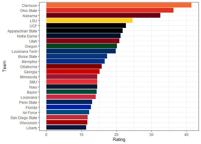
To visualize the ratings, let’s make a plot of the top 25.
library(ggplot2)
library(forcats)

srs <-
  tibble(team = fbs_teams$school,
         rating = solve(A, b),
         color = fbs_teams$color)

top_25 <-
  srs %>%
  arrange(desc(rating)) %>%
  slice(1:25)

ggplot() +
  geom_col(data = top_25, aes(x = fct_reorder(team, rating), y = rating), fill = top_25$color) +
  coord_flip() +
  theme_bw() +
  ylab("Rating") +
  xlab("Team")
In the College Football Data blog, they further refine the rating by factoring in home field advantage, conference strength, and things like that.
That fine, but I just wanted to get the basic mechanics down.


Comments