Neural Network Regression

The following is a subsection of a tutorial I co-authored that I wanted to reproduce here to work out how to get the figures to render properly. Plus, it never hurts to revisit the fundamentals.

library(tidyverse)

Neural Network Regression

Like support vector machines and tree-based models, neural networks can be applied to both regression and classification tasks. Neural networks originated in the field of neurophysiology as an attempt to model human brain activity¹ at the neuron level, but it wasn’t until the 1980s and 1990s² that they began to be developed into their current form. Neural network models are fit using a training algorithm that slowly reduces prediction error using a process called gradient descent.

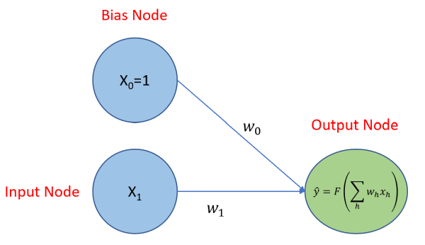
Simple Neural Network Model

Before we get into that, let’s look at visualization of a neural network regression model in it’s simplest form: one to solve for β₀ and β₁ given the equation where we know x₀ = 1. Below, the two blue circles are referred to as the input layer and consist of two nodes: an input node that will be used to solve for β₁, and a bias node to solve for β₀, the y-intercept. Each node of the input layer is connected to the output layer, which consists of just one node because we’ll be predicting a single continuous variable, . If this was a classification problem, and we were trying to classify the three types of irises found in the iris data set, then the output layer would have three nodes, each producing a probability. There is a model parameter, referred to as a weight, associated with each connected node as indicated by the ω₀ and ω₁ terms. The output node produces a prediction, , using an activation function. In the case of linear regression, we use a linear activation function of the form . That’s it - that’s the model!

Gradient Descent

The algorithm used to train the model is called gradient descent, and to demonstrate how it works, we need to set the stage first. Let’s assume that we’re trying to find the βs that have the following relationship with the predictor:

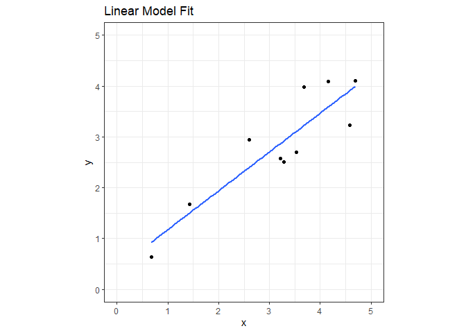
We’ll create a data set with 10 observations and fit a linear model for comparison later.

set.seed(42)
nn_reg = tibble(
  x = runif(10, 0, 5),
  y = 1 + 0.5*x + rnorm(10, sd=0.5)
)
ggplot(nn_reg, aes(x=x, y=y)) +
  geom_point() +
  geom_smooth(formula='y~x', method='lm', se=FALSE) +
  coord_fixed(xlim=c(0,5), ylim=c(0,5)) +
  ggtitle("Linear Model Fit") +
  theme_bw()

nn.lm = lm(y ~ x, data=nn_reg)
summary(nn.lm)

##
## Call:
## lm(formula = y ~ x, data = nn_reg)
##
## Residuals:
##      Min       1Q   Median       3Q      Max
## -0.67369 -0.38063 -0.08963  0.41550  0.75801
##
## Coefficients:
##             Estimate Std. Error t value Pr(>|t|)    
## (Intercept)   0.4127     0.4516   0.914 0.387494    
## x             0.7641     0.1324   5.773 0.000418 ***
## ---
## Signif. codes:  0 '***' 0.001 '**' 0.01 '*' 0.05 '.' 0.1 ' ' 1
##
## Residual standard error: 0.5164 on 8 degrees of freedom
## Multiple R-squared:  0.8064,	Adjusted R-squared:  0.7822
## F-statistic: 33.32 on 1 and 8 DF,  p-value: 0.000418

Before the model is trained, its weights are initialized with random numbers. I’ll just pick two random numbers between -1 and 1.

set.seed(42)
(w0 = runif(1, -1, 1))

## [1] 0.8296121

(w1 = runif(1, -1, 1))

## [1] 0.8741508

Since these model parameters are just random numbers, the predictions will not be very accurate. That’s ok, though, and it’s the starting point for all untrained neural network models. We’ll go through the following iterative process to slowly train the model to make more and more accurate predictions.

The Training Process

1. Make predictions for input values.
2. Measure the difference between those predictions and the true values (called the loss).
3. Compute the partial derivative (gradient) of the loss with respect to the model parameters.
4. Update the model parameters using the partial derivative values computed in the previous step.
5. Repeat this process until the loss is either unchanged or is sufficiently low.

The next several code chunks demonstrate this process one step at a time.

Step 1. Make predictions.

We can make predictions manually using the randomly initialized weight and bias.

get_estimate = function(omega0, omega1){nn_reg$x * omega1 + omega0}
(y_hat = get_estimate(w0, w1))

##  [1] 4.828004 4.925338 2.080258 4.459294 3.634524 3.098453 4.049059 1.418207
##  [9] 3.701164 3.911277

Step 2. Calculate the loss.

There are a number of ways we could do this, but for this example, we’ll calculate the loss by determining the mean squared error of the predictions and the target values. Mean squared error is defined as:

mse = function(predicted){1/length(predicted)* sum((nn_reg$y - predicted)^2)}
# the loss
(loss = mse(y_hat))

## [1] 0.8201885

Step 3. Compute the partial derivatives of the loss.

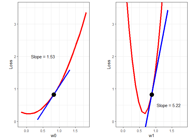
At this point, we have two random values for ω₀ and ω₁ and an associated loss (error). Now we need to find new values for the ωs that will decrease the loss. How do we do that? For each ω, we need to determine whether we should increase or decrease it’s value and by how much. We determine whether to increase or decrease its value by calculating the gradient of the loss function at the current ω values. To demonstrate graphically, the loss as a function of ω₀ and ω₁ are plotted below.

# sequence of w0 values
Bvec = seq(from=(w0-1), to=(w0+1), length.out = 21)
# calculate loss while holding w1 constant
Bloss = Bvec %>% map(function(x) get_estimate(x, w1)) %>% map_dbl(function(x) mse(x))
# get a curve through the points and get the gradient
Bspl = smooth.spline(Bloss ~ Bvec)
# get the gradient at w0
Bgrad = predict(Bspl, x=w0, deriv=1)$y
# same thing for w1
Wvec = seq(from=(w1-1), to=(w1+1), length.out = 21)
Wloss = Wvec %>% map(function(x) get_estimate(w0,x)) %>% map_dbl(function(x) mse(x))
Wspl = smooth.spline(Wloss ~ Wvec)
Wgrad = predict(Wspl, x=w1, deriv=1)$y
w0plot = ggplot() +
  geom_line(aes(x=Bvec, y=Bloss), color='red', size=1.5) +
  geom_line(aes(x=c(w0-0.5, w0+0.5), y=c(Bloss[11]-Bgrad/2, Bloss[11]+Bgrad/2)), color='blue', size=1.5) +
  geom_point(aes(x=Bvec[11], y = Bloss[11]), size=5) +
  annotate("text", x=0.5, y=2, label=paste("Slope =", round(Bgrad, 2))) +
  coord_fixed(ylim=c(0,3.5)) +
  xlab("w0") + ylab("Loss") +
  theme_bw()
w1plot = ggplot() +
  geom_line(aes(x=Wvec, y=Wloss), color='red', size=1.5) +
  geom_line(aes(x=c(w1-0.5, w1+0.5), y=c(Wloss[11]-Wgrad/2, Wloss[11]+Wgrad/2)), color='blue', size=1.5) +
  geom_point(aes(x=Wvec[11], y=Wloss[11]), size=5) +
  annotate("text", x=1.4, y=0.5, label=paste("Slope =", round(Wgrad, 2))) +
  coord_fixed(ylim=c(0,3.5)) +
  xlab("w1") + ylab("Loss") +
  theme_bw()
gridExtra::grid.arrange(w0plot, w1plot, nrow=1, ncol=2)

In practice, the partial derivatives are calculated as follows:

(Bpartial = sum(-(nn_reg$y - y_hat)))

## [1] 7.670526

(Wpartial = sum(-(nn_reg$y - y_hat) * nn_reg$x))

## [1] 26.07812

Step 4. Update the model parameters.

From the above plots, we can see that to decrease the loss, we need to decrease both ωs. In fact, the following rules always apply:

• With a positive gradient, decrease the parameter value.

• With a negative gradient, increase the parameter value.

We know we need to decrease the parameter values, so now we need to determine how much to decrease them. Right now, all we have to go on are the magnitude of the gradients. If we decreased the parameters by their respective gradients, the new parameter values would be far to the left on both plots above - we would overshoot the bottom of the curve in both cases. Instead of using the full gradient value, it appears that the parameters should be updated as follows:

Where α is a multiplier in the range [0, 1], and is referred to as the learning rate. For our example, an α of 0.01 will suffice, but keep in mind that α is a hyperparameter that often must be tuned. The code below selects α, updates the parameter values, and recalculates the loss. Notice that the loss has decreased as expected.

alpha = 0.001
w0 = w0 - Bpartial * alpha
w1 = w1 - Wpartial * alpha
mse(get_estimate(w0, w1))

## [1] 0.6816571

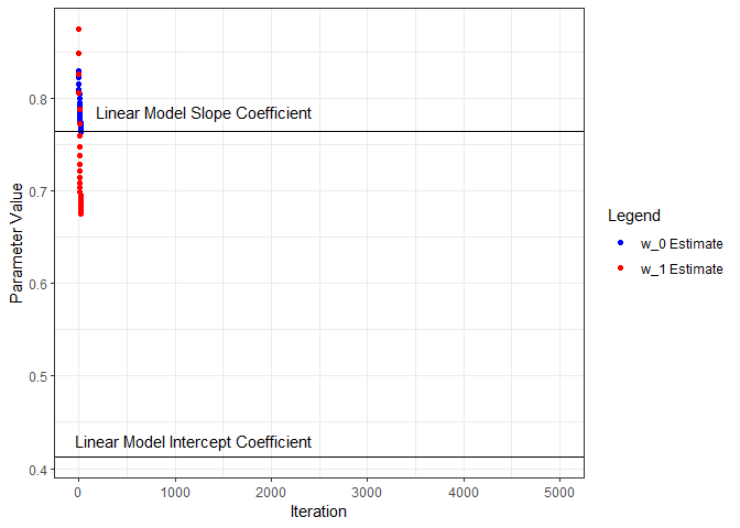
Next we’ll put all this in a loop, iterate through a number of times, and see what we get for parameter estimates. I’ll start from the beginning and capture the parameters and loss as training progresses through 5000 iterations. Below, the parameter estimates are plotted for each iteration and compared to the linear model coefficients.

set.seed(42)
w0 = runif(1, -1, 1)
w1 = runif(1, -1, 1)
alpha = 0.001
w0s = w0
w1s = w1
for (j in 1:500){
  for (i in 1:nrow(nn_reg)){
    y_hat = get_estimate(w0, w1)
    Bgrad = sum(-(nn_reg$y - y_hat))
    Wgrad = sum(-(nn_reg$y - y_hat) * nn_reg$x)
    w0 = w0 - Bgrad * 0.001
    w1 = w1 - Wgrad * 0.001
    w0s = c(w0s, w0)
    w1s = c(w1s, w1)
  }
}

wHistory = tibble(
  iter = 1:length(w0s),
  b = w0s,
  w = w1s
)

library(gganimate)

ggplot(wHistory) +
  geom_point(aes(x=iter, y=w0s, color='w_0 Estimate', group=seq_along(iter))) +
  geom_hline(yintercept=coef(nn.lm)[1]) +
  annotate("text", x=1200, y=0.43, label="Linear Model Intercept Coefficient") +
  geom_point(aes(x=iter, y=w1s, color='w_1 Estimate', group=seq_along(iter))) +
  geom_hline(yintercept=coef(nn.lm)[2]) +
  annotate("text", x=1300, y=0.785, label="Linear Model Slope Coefficient") +
  scale_color_manual(name="Legend", values=c('blue', 'red')) +
  xlab("Iteration") + ylab("Parameter Value") +
  theme_bw() +
  transition_reveal(iter)

To visualize the gradient descent methodology, calculate the loss for a range of ω₀ and ω₁ values and plot the loss function as a surface.

loss_fn = expand_grid(bs=seq(0.3,0.9,length.out=20), ws=seq(0.5,1,length.out=20))

loss_fn$Loss = 1:nrow(loss_fn) %>%
  map(function(x) get_estimate(loss_fn[x,'bs'] %>% .$bs, loss_fn[x,'ws']%>% .$ws)) %>%
  map_dbl(function(x) mse(x))

ggplot(wHistory) +
  geom_raster(data=loss_fn, aes(x=bs, y=ws, fill=Loss)) +
  geom_contour(data=loss_fn, aes(x=bs, y=ws, z=Loss), color='white', bins=28) +
  geom_point(aes(x=b, y=w, group=seq_along(iter)), color='yellow', size=5) +
  xlab("Intercept") + ylab("Slope") +
  theme_bw() +
  transition_time(iter) +
  labs(title = paste("Gradient Descent Iteration:", "{round(frame_time, 0)}")) +
  shadow_wake(wake_length = 0.2)

We can also see the regression line update as training progresses.

ggplot(wHistory) +
  geom_smooth(data=nn_reg, aes(x=x, y=y), formula='y~x', method='lm', se=FALSE) +
  geom_abline(aes(intercept=b, slope=w), color='red') +
  geom_point(data=nn_reg, aes(x=x, y=y)) +
  coord_fixed(xlim=c(0,5), ylim=c(0,5)) +
  theme_bw() +
  transition_time(iter) +
  labs(title = paste("Gradient Descent Iteration:", "{round(frame_time, 0)}"))

Let’s compare the final parameter estimates from the neural network model to the linear model coefficients.

tibble(
  Model = c("Linear", "Neural Network"),
  w_0 = c(coef(nn.lm)[1], tail(w0s, 1)),
  w_1 = c(coef(nn.lm)[2], tail(w1s, 1))
)

## # A tibble: 2 x 3
##   Model            w_0   w_1
##   <chr>          <dbl> <dbl>
## 1 Linear         0.413 0.764
## 2 Neural Network 0.414 0.764

There are a variety of R packages to simplify the process of fitting a neural network model. Since we’re doing regression and not something for complicated like image classification, natural language processing, or reinforcement learning, a package like nnet provides everything we need.

nnModel = nnet::nnet(y ~ x, data = nn_reg,   # formula notation is the same as lm()
                     linout = TRUE,          # specifies linear output (instead of logistic)
                     decay = 0.001,          # weight decay
                     maxit = 100,            # stop training after 100 iterations
                     size = 0, skip = TRUE)  # no hidden layer (covered later)

## # weights:  2
## initial  value 31.444863
## final  value 2.134476
## converged

summary(nnModel)

## a 1-0-1 network with 2 weights
## options were - skip-layer connections  linear output units  decay=0.001
##  b->o i1->o
##  0.41  0.76

From the model summary, we see that has two weights: one for ω₀ and one for ω₁. The initial and final values are model error terms. Converged means that training stopped before it reached maxit. The model takes the form 1-0-1, which means it has one input node (the bias, or intercept, node is automatically included) in the input layer, 0 nodes in the hidden layer (we’ll cover hidden layers later), and one node in the output layer. The b->o term is our ω₀ (intercept) parameter value, and i1->o is our ω₁ (slope) parameter value. We can extract the coefficients the usual way.

coef(nnModel)

##      b->o     i1->o
## 0.4125070 0.7641276

Multiple Linear Regression

The neural network model can be easily expanded to accommodate additional predictors by adding a node to the input layer for each additional predictor and connecting it to the output node. Below is a comparison of coefficients obtained from a linear model and a neural network model for a data set with three predictors.

# make up data
set.seed(42)
mlr = tibble(
  x1 = runif(10, 0, 5),
  x2 = runif(10, 0, 5),
  x3 = runif(10, 0, 5),
  y = 1 + 0.5*x1 - 0.5*x2 + x3 + rnorm(10, sd=0.5)
)

# linear model coefficients
coef(lm(y ~ ., data=mlr))

## (Intercept)          x1          x2          x3
##   2.0447549   0.5355719  -0.7312496   0.8035532

# neural network coefficients
coef(nnet::nnet(y ~ ., data = mlr, linout = TRUE, decay = 0.001, maxit = 100,
                     size = 0, skip = TRUE))

## # weights:  4
## initial  value 195.927838
## final  value 4.149504
## converged

##       b->o      i1->o      i2->o      i3->o
##  2.0399505  0.5361400 -0.7307887  0.8040190

If you think this seems like overkill just to model a linear relationship between two variables, I’d agree with you. But consider this:

• What if the relationship between two variables isn’t linear?

• What if there are dozens of predictor variables and dozens of response variables and the underlying relationships are highly complex?

In cases like these, neural networks models can be very beneficial. To make that leap, however, we need to give our neural network model more power by giving it the ability to model these complexities. We do that by adding one or more hidden layers to the model.

Hidden Layer

Neural network models become universal function approximators with the addition of one or more hidden layers. Hidden layers fall between the input layer and the output layer. Adding more predictor variables and one hidden layer, we get the following network.

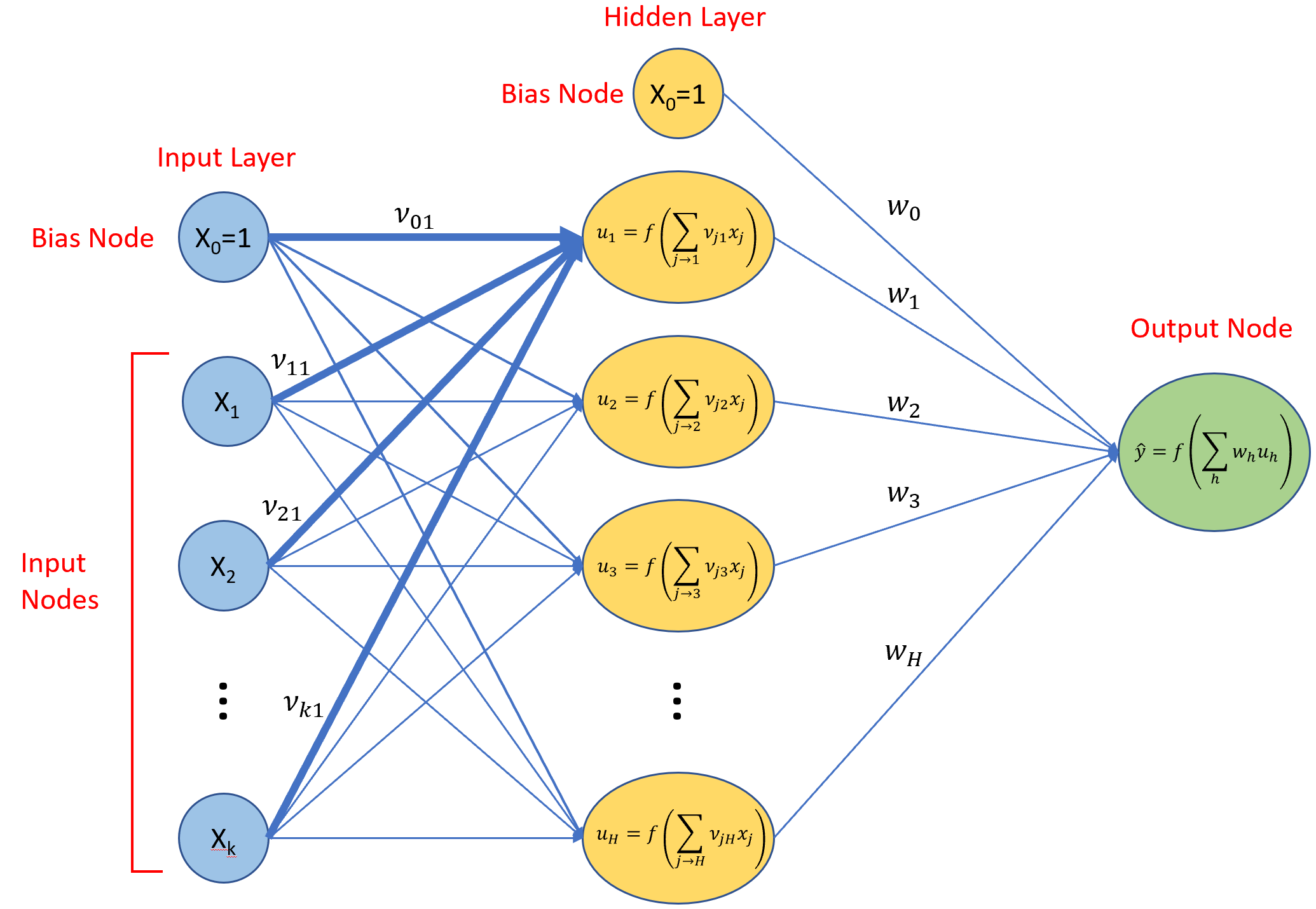
We’ve introduced a new variable ν, and a new function u. The ν variables are trainable weights just like the w variables. The u functions are activation functions as described earlier. Typically, all nodes in a hidden layer share a common type of activation function. A variety of activation functions have been developed, a few of which are shown below. For many applications, a rectified linear, activation function is a good choice for hidden layers.

Activation Function	Activation Function Formula	Output Type
Threshold		Binary
Linear		Numeric
Logistic		Numeric Between 0 & 1
Rectified Linear		Numeric Positive

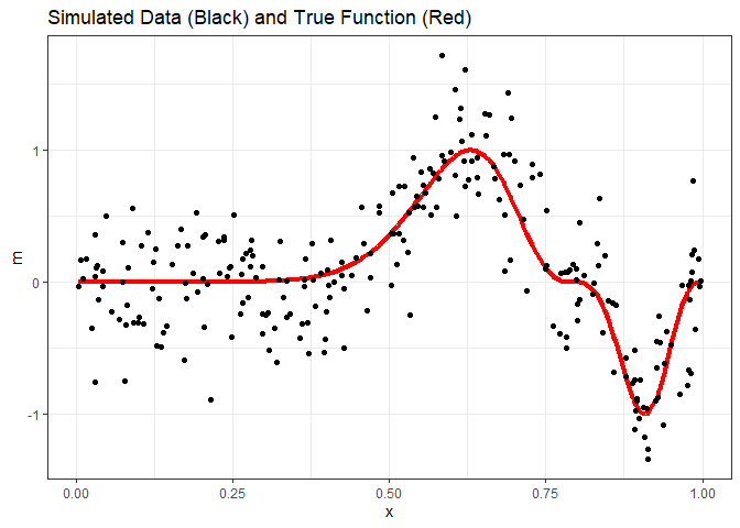
As stated, adding a hidden layer turns the neural network model into a universal function approximator. For the case of regression, we can think of this as giving the neural network the ability to model non-linear functions without knowing what the nature of the nonlinear relationship is. Compare that to linear regression. If we had the relationship y = x², we would need to transform either the response or predictor variable in a linear regression model, and this requires knowing the order of the polynomial to get a good fit. With neural network regression, we don’t need this knowledge. Instead, we allow the hidden layer to learn the nature of the relationship through the model training process. To demonstrate, we’ll use the exa data set from the faraway package, which looks like this.

exa = faraway::exa

ggplot(exa) +
  geom_line(aes(x=x, y=m), color='red', size=1.5) +
  geom_point(aes(x=x, y=y)) +
  ggtitle("Simulated Data (Black) and True Function (Red)") +
  theme_bw()

To fit a linear model with a 10-node hidden layer, we specify size = 10, and since 100 iterations might not be enough to converge, we’ll increase maxit to 500. Otherwise, everything else is the same. With 2 nodes in the input layer (1 for the bias, 1 for x) and 11 nodes in the hidden layer (1 for the bias, and 10 for those we specified), the model will have 31 weights to train.

nnModel2 = nnet::nnet(y ~ x, data = exa, linout = TRUE, decay = 10^(-4), maxit = 500, size = 10)

## # weights:  31
## initial  value 499.220789
## iter  10 value 78.378021
## iter  20 value 48.290911
## iter  30 value 40.726235
## iter  40 value 27.840931
## iter  50 value 26.694405
## iter  60 value 25.771768
## iter  70 value 25.636428
## iter  80 value 25.582253
## iter  90 value 25.475199
## iter 100 value 25.237757
## iter 110 value 24.502290
## iter 120 value 24.125822
## iter 130 value 23.715466
## iter 140 value 23.644963
## iter 150 value 23.592656
## iter 160 value 23.541215
## iter 170 value 23.460968
## iter 180 value 23.394390
## iter 190 value 23.326002
## iter 200 value 23.299889
## iter 210 value 23.294752
## iter 220 value 23.253858
## iter 230 value 23.176888
## iter 240 value 23.124385
## iter 250 value 23.104052
## iter 260 value 23.084055
## iter 270 value 23.080214
## iter 280 value 23.078985
## iter 290 value 23.076738
## iter 300 value 23.074305
## iter 310 value 23.073038
## iter 320 value 23.072321
## final  value 23.071986
## converged

preds = predict(nnModel2, newdata=data.frame(x=exa$x))

ggplot() +
  geom_line(data=exa, aes(x=x, y=m, color='True Function'), size=1.5) +
  geom_line(aes(x=exa$x, y=preds, color='Model Fit'), size=1.5) +
  geom_point(data=exa, aes(x=x, y=y)) +
  scale_color_manual(name="Legend", values=c('blue', 'red')) +
  theme_bw()

The plot above indicates the model over fit the data somewhat, although we only know this because we have the benefit of knowing the true function. We could reduce the amount of over fitting by choosing different hyperparameter values (decay, or the number of hidden layer nodes) or by changing the default training stopping criteria.

The trained model’s weights are saved with the model, and all 31 are shown below. This highlights a significant drawback of neural network regression. Earlier when we used a neural network model to estimate the slope and intercept, the model weights had meaning: we could directly interpret the weights as slope and intercept. How do we interpret the weights below? I have no idea! The point is that neural network models can be trained to make highly accurate predictions…but at the cost of interpretability.

nnModel2$wts

##  [1] -16.5006608  20.3693099 -29.4278236  34.4051715 -20.7471248  28.4091270
##  [7] -29.1180265  40.7327613   2.3060868   1.9215748  -1.0624319   2.9527926
## [13]   2.8259165 -15.1652645   1.6957639   0.5958946   3.7441769 -21.0803998
## [19]   6.3092685  -8.3407380   1.3998851  19.2726000 -11.2056916 -23.2575100
## [25]   9.5932587   2.2295197   3.1400221   6.4367782   0.4575623  -4.5860998
## [31]  -6.2028427

Neural Network Classification

Neural network models have been extremely successful when applied to classification tasks such as image classification and natural language processing. These models are highly complex and are built using sophisticated packages such as TensorFlow (developed by Google) and PyTorch (developed by Facebook). Building complex models for those kinds of classification tasks are beyond the scope of this tutorial. Instead, this section provides a high-level overview of classification using the nnet package and the iris data set.

The neural network training algorithm for classification is the same as for regression, but for classification, we need to change some of the attributes of the model itself. Instead of a linear activation function in the output layer, we need to use the softmax function. Doing so will cause the output layer to produce probabilities for each of the three flower species (this is accomplished by simply removing linout = TRUE from the nnet() function. Additionally, we use a categorical cross entropy loss function instead of mean squared error. Below, I also set rang = 0.1 to scale the predictors to be in the range recommended in the function help. We’ll also create the same training/test split as in the non-parametric regression chapter so we can directly compare results.

# create a training and a test set
set.seed(0)
train = caTools::sample.split(iris, SplitRatio = 0.8)
iris_train = subset(iris, train == TRUE)
iris_test = subset(iris, train == FALSE)

# train the model
irisModel = nnet::nnet(Species ~ ., data = iris_train,
                       size=2,       # only two nodes in the hidden layer
                       maxit=200,    # stopping criteria
                       entropy=TRUE, # switch for entropy
                       decay=5e-4,   # weight decay hyperparameter
                       rang=0.1)     # scale input values

## # weights:  19
## initial  value 131.916499
## iter  10 value 75.933787
## iter  20 value 56.873818
## iter  30 value 55.958531
## iter  40 value 55.852468
## iter  50 value 55.797951
## iter  60 value 51.382669
## iter  70 value 11.286807
## iter  80 value 7.667108
## iter  90 value 7.657444
## iter 100 value 7.643547
## iter 110 value 7.642436
## iter 120 value 7.641672
## iter 130 value 7.640995
## iter 140 value 7.640338
## iter 150 value 7.627436
## iter 160 value 7.377487
## iter 170 value 5.671710
## iter 180 value 4.882362
## iter 190 value 4.810287
## iter 200 value 4.793128
## final  value 4.793128
## stopped after 200 iterations

# make predictions on test data
iris_preds = predict(irisModel, newdata=iris_test)
head(iris_preds)

##       setosa  versicolor    virginica
## 5  0.9956710 0.004329043 6.376970e-16
## 10 0.9911190 0.008881042 2.881866e-15
## 15 0.9976175 0.002382547 1.824318e-16
## 20 0.9957198 0.004280170 6.226948e-16
## 25 0.9739313 0.026068739 2.794827e-14
## 30 0.9901521 0.009847885 3.581197e-15

This first six predictions for the test set are shown above, and notice that the values are in fact probabilities. The model is highly confident that each one of these first six predictions are setosa. Recall from the SVM and CART sections of the non-parametric regression chapter that both of those models misclassified test set observations #24 and #27 as versicolor that are actually virginica. Below we see that the neural network model correctly predicts both observations but is less confident about observation #24.

iris_preds[c(24,27), ]

##           setosa versicolor virginica
## 120 7.349090e-11 0.18967040 0.8103296
## 135 5.460005e-13 0.03105806 0.9689419

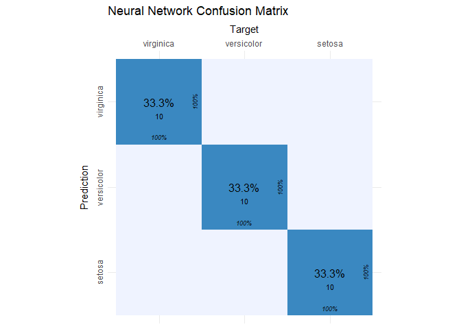
The confusion matrix for the entire test set reveals that the model has an accuracy of 100%.

iris_cm = cvms::confusion_matrix(
  targets = iris_test[, 5],
  predictions = colnames(iris_preds)[max.col(iris_preds)])

cvms::plot_confusion_matrix(iris_cm$`Confusion Matrix`[[1]], add_zero_shading = FALSE) +
  ggtitle("Neural Network Confusion Matrix")

1. Warren S. McCulloch, Walter H. Pitts. 1943. “A Logical Calculus of the Ideas Immanent in Nervous Activity.” Bulletin of Mathematical Biophysics 5. ↩

2. David E. Rumelhart, James L. McClelland. 1986. Parallel Distributed Processing. MIT Press. Bishop, Christopher. 1995. Neural Networks for Pattern Recognition. Oxford University Press. ↩