The Recaman Sequence

The next stop on my generative art journey took me to the Recaman Sequence. As opposed to many other algorithms, there’s no randomness in this sequence - the sequence is what it is. At some point, someone much more clever than me figured out an interesting way to visualize it. First, I’ll describe the sequence, then the visualization technique.

The Recaman Sequence

The Wikipedia entry states that, to generate the Recaman sequence, apply the following algorithm.

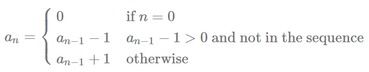
In English, that means we make a counter n that starts at 1 and goes up. For each counter number, we’re going to try to go backwards that many positions in the sequence. If that position in the sequence doesn’t exist or if that position already has a value in it, then we go forward that many positions.

Besides the counter, we also need to keep track of the sequence itself, which starts at 0. Let’s consider that a moment. We have a counter that starts at 1, and a sequence that starts at 0. Indexing in R starts at 1, so we need to be really careful not to get an off-by-one error (OOBE)! If we’re careful, we should end up with the following first few numbers in the sequence [0, 1, 3, 6, 2, 7].

So, time to give it a shot and generate the first six numbers. So I didn’t commit the OOBE, I actually re-wrote the rules above by hand and walked through the rules. From that exercise, I found that instead of the +1 and -1 terms, I need +[n-1] and -[n-1]. This code does the trick.

a <- 0

for (n in 1:1000){
  ifelse(a[n - 1] - (n - 1) > 0 & !(a[n - 1] - (n - 1)) %in% a,
         a <- c(a, a[n - 1] - (n - 1)),
         a <- c(a, a[n - 1] + (n - 1)))
}

a[1:6]

## [1] 0 1 3 6 2 7

That’s really all there is to it. All we need to do is just expand that sequence out however long we want.

Data Visualization

As I said earlier, I think this is the clever bit. The way this works is that we connect each number in the sequence with a half-circle that alternates between arching above and arching below a horizontal line. To do that, I wrote this function. It takes two adjacent numbers from the sequence and creates 33 (x, y) coordinates that, when connected together with a line, will make a half circle. There’s some logic built in to handle the need to alternate up and down, and also the difference between arcing to the right on the horizontal line between 1 and 3 versus arcing to the left between 6 and 3.

generate_circle_points <- function(idx, p1, p2){
  radius <- (p2 - p1) /2
  x <- radius
  y <- 0
  for (alpha in 1:32 * 180/32 * pi/180){
    x <- c(x, radius * cos(alpha))
    y <- c(y, radius * sin(alpha))
  }
  if (idx %% 2 != 0){y <- -y}   # logic for up/down
  if (p1 > p2){y <- -y}         # logic for left/right
  x <- rev(x)
  data.frame(x = x + radius + p1, y = y)
}

Now we iterate though the sequence and create all of the half circles.

for (i in 1:(length(a) - 1)){
  if(i == 1){
    df <- generate_circle_points(i, a[i], a[i+1])
    df$arc <- i
  }else{
    df_new <- generate_circle_points(i, a[i], a[i+1])
    df_new$arc <- i
    df <- rbind(df, df_new)
  }
}

head(df)

##             x           y arc
## 1 0.000000000  0.00000000   1
## 2 0.002407637 -0.04900857   1
## 3 0.009607360 -0.09754516   1
## 4 0.021529832 -0.14514234   1
## 5 0.038060234 -0.19134172   1
## 6 0.059039368 -0.23569837   1

library(plotly)
library(RColorBrewer)


p <- df %>% mutate(arc = factor(arc)) %>%
  plot_ly() %>%
  add_paths(x=~x, y=~y, hoverinfo = "none", showlegend = FALSE,
            line = list(width = 0.5),
            color=~arc, colors = colorRampPalette(brewer.pal(10, "Spectral"))(nrow(df))) %>%
  layout(
    xaxis = list(
      title = "",
      zeroline = FALSE,
      showline = FALSE,
      showticklabels = FALSE,
      showgrid = FALSE),
    yaxis = list(
      title = "",
      zeroline = FALSE,
      showline = FALSE,
      showticklabels = FALSE,
      showgrid = FALSE,
      scaleanchor = "x",
      scaleratio = 1
    ),
    paper_bgcolor = "#000000", plot_bgcolor = "#000000")

p

You can click here for my Shiny app to generate your own art using this and other algorithms.