Driving Up A Mountain

A while back, I found OpenAI’s Gym environments and immediately wanted to try to solve one of their environments. I didn’t really know what I was doing at the time, so I went back to the basics for a better understanding of Q-learning and Deep Q-Networks. Now I think I’m ready to graduate from tic-tac-toe and try a Gym environment again. Best to start simple, though.

The Mountain Car Environment

There are two Mountain Car environments: one with a discrete number of actions, and one with a continuous range of actions. Keeping it simple means go with the discrete case. The Gym documentation describes the situation and the goal:

A car is on a one-dimensional track, positioned between two “mountains”. The goal is to drive up the mountain on the right; however, the car’s engine is not strong enough to scale the mountain in a single pass. Therefore, the only way to succeed is to drive back and forth to build up momentum.

One of the nice things about working with Gym environments is that I don’t have to put effort into defining my own environment like I did with tic-tac-toe. All I have to do to create the mountain car environment is gym.make('MountainCar-v0'). It’s that easy! I need to get some information about the state space and actions so I know what I’m dealing with. First the state space.

import gym
env = gym.make('MountainCar-v0')
print(env.observation_space)

Box(2,)

Box means that it’s a continuous state space, and the 2 means there are two numbers that represent the space. Going back to the documentation, the state represents the position and velocity of the car. I can get their upper and lower bounds this way:

print(env.observation_space.high)

[0.6  0.07]

print(env.observation_space.low)

[-1.2  -0.07]

So the car’s position can be between -1.2 and 0.6, and the velocity can be between -0.07 and 0.07. The documentation states that an episode ends the car reaches 0.5 position, or if 200 iterations are reached. That means the position value is the x-axis with positive values to the right, and that a positive velocity means the car is moving to the right. The documentation also says that the starting state is a random position from -0.6 to -0.4 with no velocity, so I start at the bottom of the value at a stand still. Makes sense. What do I have for actions?

print(env.action_space)

Discrete(3)

Three possible actions. 0 means push left, 1 means do nothing (not sure why you’d ever do that), and 2 means push right.

Last thing I need is how the rewards work. They say you get “-1 for each time step until the goal position of 0.5 is reached”. So there’s no positive reward? Huh. They also say “there is no penalty for climbing the left hill, which upon reached acts as a wall”. I guess that means I can bounce my car off it.

To interact with the environment, I first need to reset it with env.reset(). This gives me the car’s starting state. Then I need an action. I can get a random action from the environment with env.action_space.sample(), or I could just use numpy to generate a random number. Anyway, then to execute that action in the environment, I use env.step(action). This returns the next observation based on that action, the reward (always -1), whether the episode is over, and some empty information. Also according to the docs, I should close the environment when I’m done with it. Here I’ll take 5 random actions to see what things look like.

observation = env.reset()
print("observation:", observation)
for t in range(5):
    action = env.action_space.sample()
    print("action:", action)
    observation, reward, done, info = env.step(action)
    print("step results:", observation, reward, done, info)
env.close()

observation: [-0.44439613  0.        ]
action: 2
step results: [-4.43984578e-01  4.11553896e-04] -1.0 False {}
action: 1
step results: [-4.4416447e-01 -1.7989169e-04] -1.0 False {}
action: 0
step results: [-0.4459345  -0.00177003] -1.0 False {}
action: 1
step results: [-0.44828175 -0.00234725] -1.0 False {}
action: 2
step results: [-0.45018908 -0.00190734] -1.0 False {}

Ok, got it. I’ll import a bunch of stuff and then get to solving this thing with a DQN agent.

import numpy as np
import tensorflow as tf
from tensorflow import keras
from collections import deque

%matplotlib inline
import matplotlib as mpl
import matplotlib.pyplot as plt
mpl.rc('axes', labelsize=14)
mpl.rc('xtick', labelsize=12)
mpl.rc('ytick', labelsize=12)

# To get smooth animations
import matplotlib.animation as animation
mpl.rc('animation', html='jshtml')

try:
    import pyvirtualdisplay
    display = pyvirtualdisplay.Display(visible=0, size=(1400, 900)).start()
except ImportError:
    pass

DQN Agent

If you read my last post on Deep Q-Networks, a lot of this will look familiar. I’m only going to explain what’s different, so you might want to go back and read it.

build_model: The only thing I changed here was to reduce the number of nodes in the two hidden layers. Since there are only two values that represent the state and only three actions, 32 nodes seemed plenty.

add_memory: This is completely new. What I’m doing here is storing information about every step (an “experience”) to create what’s referred to as a replay memory. In the __init__ function, I create a deque of length 2000 for this purpose. This function simply adds an experience to the replay memory. Since it’s a deque, once it contains 2000 items, adding a new item to the top of the queue will cause the oldest item to be removed.

sample_experiences: This is also new and is part of the replay memory implementation. This function is called only after the replay memory deque is full. Here I randomly sample 64 experiences (defined by batch_size) from the replay memory. According to Aurélien Géron,

This helps reduce the correlations between the experiences in a training batch, which tremendously helps training.

train_model: The only thing different here is the implementation of training from memory replay via self.sample_experiences() instead of training based on the full set of experiences. Otherwise, the neural net is trained exactly the same way as it did for the tic-tac-toe example. Although not strictly part of this function, I also switched from a stochastic gradient decent optimizer to an Adam optimizer and decreased the learning rate to 0.001 in the __init__ function.

class DQNagent:

    def __init__(self, state_size, action_size, episodes):
        self.gamma = 0.95
        self.batch_size = 64
        self.state_size = state_size
        self.action_size = action_size
        self.episodes = episodes
        self.replay_memory = deque(maxlen=2000)
        self.optimizer = tf.keras.optimizers.Adam(lr=0.001)
        self.loss_fn = tf.keras.losses.mean_squared_error

    def build_model(self):
        model = tf.keras.models.Sequential([
            tf.keras.layers.Dense(32, activation="relu", input_shape=[self.state_size]),
            tf.keras.layers.Dense(32, activation="relu"),
            tf.keras.layers.Dense(self.action_size)
        ])
        return model

    def add_memory(self, state, action, reward, next_state, done):
        self.replay_memory.append((state, action, reward, next_state, done))

    def sample_experiences(self):
        indices = np.random.randint(len(self.replay_memory), size=self.batch_size)
        batch = [self.replay_memory[index] for index in indices]
        states, actions, rewards, next_states, dones = [
            np.array([experience[field_index] for experience in batch])
            for field_index in range(5)]
        return states, actions, rewards, next_states, dones

    def train_model(self, model):
        states, actions, rewards, next_states, dones = self.sample_experiences()
        next_Q_values = model.predict(next_states)
        max_next_Q_values = np.max(next_Q_values, axis=1)
        target_Q_values = (rewards + (1 - dones) * self.gamma * max_next_Q_values)
        target_Q_values = target_Q_values.reshape(-1, 1)
        mask = tf.one_hot(actions, self.action_size)
        with tf.GradientTape() as tape:
            all_Q_values = model(states)
            Q_values = tf.reduce_sum(all_Q_values * mask, axis=1, keepdims=True)
            loss = tf.reduce_mean(self.loss_fn(target_Q_values, Q_values))
        grads = tape.gradient(loss, model.trainable_variables)
        self.optimizer.apply_gradients(zip(grads, model.trainable_variables))

Let The Training Begin

This problem kicked my butt for quite a while. I could not get that stupid car up the hill! It seemed so simple, but I was stumped. I actually solved this early on with a simple hard-coded policy: if the car is moving left (a negative velocity), push left. Otherwise, push right. Done. Didn’t even need a neural net, q-learning, or anything. So why bother with solving this with reinforcement learning? I guess in the real world, I wouldn’t, but the point here is to see if I can train a neural net (NN) to learn that policy.

I Tried A Lot Of Things That Didn’t Work

First, I left everything as is, and just fed experiences to the NN hoping it would learn. Recall that each episode consists of 200 steps, and so you get a -1 reward for each step for a total reward of -200. If the car reaches the goal in say 150 steps, then you get a total reward of -150. My idea here was that the NN would learn to maximize the total reward by finishing in under 200 steps. Nope. Never happened. The car never got to the goal during training and so the NN never learned anything.

Then I started thinking about the reward system. It seemed like I needed to give the NN some positive reward to encourage it along. I tried giving a small positive reward if the car made it some distance away from the range of possible starting points. That ended up teaching the NN to drive up and down the same side of the hill over and over. Clearly, the statement, “the only way to succeed is to drive back and forth to build up momentum” is correct, but how do I do that? I tried a one-time positive reward on one side of the hill and only gave additional rewards if the car then tried going up the other side of the hill. That didn’t work, either. I tried giving a huge reward if the car ever made it to the goal position, hoping that would back-propogate quickly through the NN weights. Still nope.

It seemed like this reward system I was creating was getting a lot more complicated that it should need to be, so then I tried all of the above while at the same time adjusting the tuning parameters: learning rate, discount rate, and epsilon. No luck. I tried fiddling with how the NN was constructed: number of hidden layers, nodes, etc. Nope. I also tried changing the replay memory batch size. I even took memory replay completely out of the algorithm thinking that maybe that rare time the car made it to the goal kept getting missed in the random draw from the memory replay. Nope again.

What Did Work

It dawned on me that maybe I should just come up with a reward system that mimiced the hard-coded policy I described earlier. Finally, that worked! In the code below, you’ll see:

• if next_state[0] - state[0] > 0 and action == 2: reward = 1 moving right and pushing right = a reward
• if next_state[0] - state[0] < 0 and action == 0: reward = 1 moving left and pushing left = a reward

The following code trans the NN for 600 epsodes and keeps track of the best score. I define the score as the number of steps it takes to reach the goal, so the fewer, the better. When a new best score is reached, I save the model weights as best_weights. After the 600th episode is over, I reset the model weights with the best weights. Why? It turns out that learning is hard, and forgetting is easy, which I’ll demonstrate shortly.

best_score = 200
episodes = 600
env = gym.make('MountainCar-v0')
state_size = env.observation_space.shape[0]
action_size = env.action_space.n
agent = DQNagent(state_size, action_size, episodes)
model = agent.build_model()
rewards = []

for episode in range(episodes):
    state = env.reset()    
    for step in range(200):
        epsilon = max(1 - episode/(episodes*0.8), 0.01)
        if np.random.rand() < epsilon: action = np.random.randint(action_size)
        else: action = np.argmax(model.predict(state[np.newaxis])[0])
        next_state, reward, done, info = env.step(action)
        if next_state[0] - state[0] > 0 and action == 2: reward = 1
        if next_state[0] - state[0] < 0 and action == 0: reward = 1        
        agent.add_memory(state, action, reward, next_state, done)
        state = next_state.copy()
        if done:
            break
    rewards.append(step)
    if step < best_score:
        best_weights = model.get_weights()
        best_score = step
    print("\rEpisode: {}, Best Score: {}, eps: {:.3f}".format(episode, best_score, epsilon), end="")
    if episode > 50:
        agent.train_model(model)

model.set_weights(best_weights)

env.close()

Episode: 51, Best Score: 199, eps: 0.894WARNING:tensorflow:Layer dense is casting an input tensor from dtype float64 to the layer's dtype of float32, which is new behavior in TensorFlow 2.  The layer has dtype float32 because it's dtype defaults to floatx.

If you intended to run this layer in float32, you can safely ignore this warning. If in doubt, this warning is likely only an issue if you are porting a TensorFlow 1.X model to TensorFlow 2.

To change all layers to have dtype float64 by default, call `tf.keras.backend.set_floatx('float64')`. To change just this layer, pass dtype='float64' to the layer constructor. If you are the author of this layer, you can disable autocasting by passing autocast=False to the base Layer constructor.

Episode: 599, Best Score: 82, eps: 0.0103

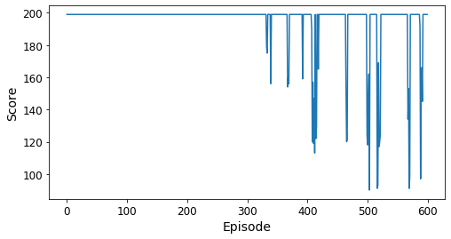
In this figure, you can see that it took about 330 episodes for the car to reach the goal for the first time. As training progressed, the score improved for a short time but then went back to 200. That happened a number of times, too. This is what Aurélien Géron describes as “catastrophic forgetting”, which makes me laugh but describes it perfectly.

According to the documentation for this environment, MountainCar-v0 is considered “solved” when the agent obtains an average reward of at least -110.0 over 100 consecutive episodes. That would translate into a score of 110 or less over 100 episodes. The best score here was 82, and looking at the graph, the NN didn’t maintain anything less than 200 very long, so there’s still work to do. I’ll go with what I have for now and demonstrate how the NN does visually.

plt.figure(figsize=(8, 4))
plt.plot(rewards)
plt.xlabel("Episode", fontsize=14)
plt.ylabel("Score", fontsize=14)
plt.show()

I swiped these functions from Aurélien Géron’s book to render the interaction with the environment in a Jupyter Notebook. Why re-invent the wheel?

def render_policy_net(model, n_max_steps=200, seed=42):
    frames = []
    env = gym.make('MountainCar-v0')
    env.seed(seed)
    np.random.seed(seed)
    obs = env.reset()
    for step in range(n_max_steps):
        frames.append(env.render(mode="rgb_array"))
        action = np.argmax(model.predict(obs[np.newaxis])[0])
        obs, reward, done, info = env.step(action)
        if done:
            break
    env.close()
    return frames

def update_scene(num, frames, patch):
    patch.set_data(frames[num])
    return patch,

def plot_animation(frames, repeat=False, interval=40):
    fig = plt.figure()
    patch = plt.imshow(frames[0])
    plt.axis('off')
    anim = animation.FuncAnimation(
        fig, update_scene, fargs=(frames, patch),
        frames=len(frames), repeat=repeat, interval=interval)
    plt.close()
    return anim

This will render in a Jupyter notebook, but I’m not sure how it’ll look here. I’m about to find out.

frames = render_policy_net(model)
plot_animation(frames)

</input>

Once Loop Reflect

Now I’ll train for 2000 episodes and see how things look.

best_score = 200
episodes = 2000
env = gym.make('MountainCar-v0')
state_size = env.observation_space.shape[0]
action_size = env.action_space.n
agent = DQNagent(state_size, action_size, episodes)
model = agent.build_model()
rewards = []

for episode in range(episodes):
    state = env.reset()    
    for step in range(200):
        epsilon = max(1 - episode/(episodes*0.8), 0.01)
        if np.random.rand() < epsilon: action = np.random.randint(action_size)
        else: action = np.argmax(model.predict(state[np.newaxis])[0])
        next_state, reward, done, info = env.step(action)
        if next_state[0] - state[0] > 0 and action == 2: reward = 1
        if next_state[0] - state[0] < 0 and action == 0: reward = 1        
        agent.add_memory(state, action, reward, next_state, done)
        state = next_state.copy()
        if done:
            break
    rewards.append(step)
    if step < best_score:
        best_weights = model.get_weights()
        best_score = step
    print("\rEpisode: {}, Best Score: {}, eps: {:.3f}".format(episode, best_score, epsilon), end="")
    if episode > 50:
        agent.train_model(model)

model.set_weights(best_weights)

env.close()

Episode: 51, Best Score: 199, eps: 0.968WARNING:tensorflow:Layer dense is casting an input tensor from dtype float64 to the layer's dtype of float32, which is new behavior in TensorFlow 2.  The layer has dtype float32 because it's dtype defaults to floatx.

If you intended to run this layer in float32, you can safely ignore this warning. If in doubt, this warning is likely only an issue if you are porting a TensorFlow 1.X model to TensorFlow 2.

To change all layers to have dtype float64 by default, call `tf.keras.backend.set_floatx('float64')`. To change just this layer, pass dtype='float64' to the layer constructor. If you are the author of this layer, you can disable autocasting by passing autocast=False to the base Layer constructor.

Episode: 1999, Best Score: 107, eps: 0.010

plt.figure(figsize=(8, 4))
plt.plot(rewards)
plt.xlabel("Episode", fontsize=14)
plt.ylabel("Score", fontsize=14)
plt.show()

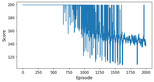
This is much better than the previous results! The NN held a sub-200 score for quite a few episodes towards the end of training. However, the best score was only 107, so there’s still more work to do to maintain sub 110 for 100 episodes. There is no incentive for reaching to goal quickly, so maybe I can get better results by adding a large reward for finishing in fewer than 110 steps. The problem with that approach is that training is conducted on a random sampling of 64 experiences out of the 2000 that are in the replay memory deque. Sub-110 scores are rare, so the chances of that reward making it into the training set is remote. Probably a better approach is to improve the NN performance so that sub-110 scores are more common. That might be possible by playing around with tuning parameters or maybe switching to a different type of reinforement learning method like a Dueling Deep Q-Network or a Double Dueling Deep Q-Network. That’s for another post, though.